Group 1
| Member | Reg.No. |
|---|---|
| 1. Saif El-Deen Ibrahim abdelslaam | 25110322 |
| 2. Mohamed Ashraf Elsayed | 25110327 |
| 3. Halla Nagi | 25110505 |
| 4. Nourhan Nagi | 25110504 |
| 5. Noor El-Shimi | 25110311 |
Guide: Match each member with the registration number in the same row. These are the five authors of this project.
Statistical analysis
Account balances,
customer behavior.
60 customers across four cities. Ten questions covering account balances, ATM use, bank services, debit-card ownership and prediction.
Average balance by city
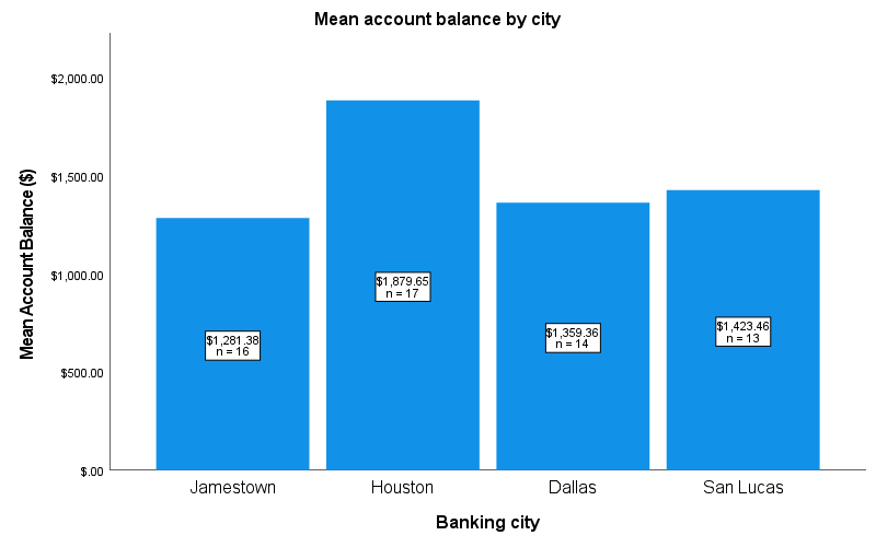
Guide: Compare bar heights on the dollar axis, not numeric city codes. Explanation: Houston has the highest sample mean. Use Q8's Welch/Games-Howell results to determine whether observed differences are statistically significant.
- Customers
- 60
- Cities
- 4
- Mean balance
- $1,499.87
- Balance–ATM correlation
- .705
- Regression R²
- 54.5%
Consolidated results summary
| Question | Method | Key results | Conclusion |
|---|---|---|---|
| Q1 | Descriptive means | Highest: Houston $1,879.65; lowest: Jamestown $1,281.38. | Descriptive comparison; significance is tested in Q8. |
| Q2 | ATM descriptives | Highest mean: Houston 11.29; largest SD: San Lucas 5.82. | Houston has the highest average ATM use; San Lucas has the greatest spread. |
| Q3 | Welch t-test | t(56.424) = -2.153; p = .036; difference = -$264.05. | Reject H0. The interest group has a higher mean balance. |
| Q4 | One-sample t-test; Wilcoxon check | Mean = 4.42; t(59) = -10.122; p < .001. Wilcoxon p < .001. | Reject the mean-equals-7 hypothesis. Average services used is below 7. |
| Q5 | Pearson chi-square | Chi-square(3) = 0.224; p = .974; Cramer's V = .061. | Fail to reject H0. No city-debit association is detected. |
| Q6 | Mann-Whitney U; Welch check | U = 415.000; p = .687. Welch mean comparison p = .326. | Fail to reject both null hypotheses. No balance difference is detected. |
| Q7 | One-sample t-test | Mean = $1,499.87; t(59) = -6.490; p < .001. | Reject the mean-equals-$2,000 hypothesis. Mean balance is below $2,000. |
| Q8 | Welch ANOVA; Games-Howell | F(3, 28.026) = 6.521; p = .002. Houston-Jamestown p = .002. | Reject H0. Houston exceeds Jamestown; no other pair is significant. |
| Q9 | Pearson correlation | r = .705; p < .001; n = 60; simple-model R squared = .497. | Strong positive linear association between balance and ATM use. |
| Q10 | Multiple regression | R squared = .545; F(2, 57) = 34.200; p < .001. Predicted balance = $1,916.93. | The model is significant; the prediction is an estimated mean, not a guaranteed balance. |
Guide: Read each question's method, result and conclusion together. Tests use a .05 significance level. Q1-Q2 are descriptive. The Q3 difference is no interest minus interest. In Q6, Mann-Whitney tests distributions and Welch tests means. Q10 predicts at 15 ATM transactions and 4 other services. Failing to reject H0 does not prove equality or independence; associations do not establish causation.
Variable definitions and numeric labels
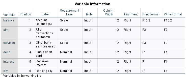
Guide: Read Variable, Label, Measurement Level and format columns; value labels are shown in the next table. Explanation: All six variables are numeric; balance, ATM use and services are scale variables. Debit, interest and city are nominal codes, not numeric magnitudes.
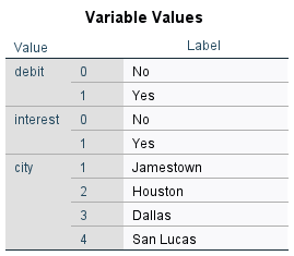
Guide: Match each numeric code to its value label before interpreting groups. Explanation: Debit/interest use 0 = No and 1 = Yes; cities use 1 = Jamestown, 2 = Houston, 3 = Dallas and 4 = San Lucas.
Lecture 3 mean precision checks
The course rule requires mean / SD at least 2.5 and mean / SE at least 10. SD describes customer spread; SE = SD / square root of n describes sample-mean precision.
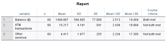
Guide: Compare Mean / SD with 2.5 and Mean / SE with 10; both must meet the lecture rule. Explanation: Balance meets both (2.513, 19.464). ATM use (2.438, 18.884) and services (2.234, 17.305) miss the SD criterion, not the SE criterion. This heuristic does not invalidate their data or determine test validity.
This is a relative-variation/precision heuristic that depends on the measurement origin and scale, not a universal test of validity. ATM/service medians and distributions remain informative; the rule does not replace normality checks, confidence intervals or the required question-specific tests.
Lecture technique coverage
Lecture 1 Data types and descriptive statistics
Included. Variable definitions distinguish three scale variables from three numerically coded nominal variables. Q2 reports mean, median, all tied modes, SD, range, minimum and maximum. Explore output provides SE, variance and distribution summaries where relevant.
Lecture 2 Charts in Excel
Included; selected chart forms. Q1 uses a mean bar chart; Q5 a grouped frequency bar chart; Q9 an Excel scatterplot and fitted straight line. Bars compare nominal categories without treating city codes as quantities. Time-trend, pie and 3-D variants are discussed in the exclusions.
Lecture 3 Validity of the mean: SD and SE checks
Added after full audit. The appendix calculates mean/SD and mean/SE for balance, ATM use and other services, with native SPSS output. Course thresholds are 2.5 and 10. This is a relative-variation/precision heuristic, not a formal normality test or a condition that determines whether a t-test is valid.
Lecture 4 Pearson correlation, direction and strength
Included. Q9 calculates Pearson r in Excel and checks it in SPSS. The scatterplot supports a positive approximately linear relationship; r = .70499 is strong under the lecture's classification. Correlation does not establish causation.
Lecture 5 Simple and multiple linear regression
Included. Q9 shows the simple linear trendline and its R-squared as a descriptive companion to correlation. Q10 fits the required two-predictor model, reports coefficients and model fit, and predicts balance at 15 ATM transactions and four services. The trendline is not substituted for multiple regression.
Lecture 6 Excel correlation and regression examples
Included. Q9/Q10 retain live CORREL and LINEST formulas, coefficient SEs, t tests, CIs, model F, R-squared, adjusted R-squared and residual SE. The equation and requested prediction are explained alongside SPSS output for the same fitted model.
Lecture 7 Hypotheses, significance and inference
Included. Each inferential question states its null and alternative hypotheses and uses alpha = .05. Decisions use p-values and, where available, confidence intervals. A non-significant result means failure to reject, not proof that populations are identical.
Lecture 8 SPSS setup, frequencies, Explore and normality plots
Included. Variable definitions and numeric value labels are shown. Descriptives, normality tests, histograms, boxplots and Q-Q plots accompany relevant analyses; Q10 adds residual diagnostics. Duplicated stem-and-leaf and menu screenshots are addressed in the exclusions.
Lecture 9 Parametric/nonparametric test selection
Included. Selections use measurement scale, independent-group count, the requested hypothesis and distribution/variance checks. Mean-based tests and rank-based sensitivity analyses are distinguished; rank tests do not automatically test population means.
Lecture 10 One-sample and independent-samples t-tests
Included; paired form excluded. Q4 tests services against seven and Q7 balance against $2,000. Q3 compares interest groups using Welch's row; Q6 includes a Welch sensitivity test of means. No specified question involves the same outcome measured twice on a customer.
Lecture 11 One-way ANOVA, post-hoc tests and uncertainty charts
Included; repeated-measures form excluded. Q8 contains ordinary ANOVA, Levene, primary Welch ANOVA, Games-Howell and a mean chart with individual 95% CIs. Tukey is replaced because variances differ. Repeated-measures ANOVA and sphericity checks require repeated outcomes absent here.
Lecture 12 Factorial ANOVA and interaction
Supplementary two-way analysis. City-by-debit Type III two-way ANOVA adds cell descriptives, normality, Levene, partial eta-squared, estimated marginal/cell means and an interaction profile. It is exploratory because variances differ. Reasons for excluding a full three-way model and extra pooled-variance follow-ups are given below.
Lecture 13 Mixed-design ANOVA
Excluded: study design does not match. No within-customer repeated outcome or time factor is supplied. Balance, ATM counts and service counts are different attributes, not occasions of the same outcome. Mixed ANOVA cannot answer the specified questions.
Lecture 14 Wilcoxon, Mann-Whitney and Kruskal-Wallis
Included; related-sample forms excluded. Q4 includes one-sample Wilcoxon and signed-rank output. Q6 includes Mann-Whitney ranks, U test and boxplot. Q8 includes Kruskal-Wallis ranks, H test, Bonferroni pairwise table and rank diagram. Paired Wilcoxon/Friedman require comparable repeated outcomes absent here.
Lecture 15 Categorical association and related binary tests
Chi-square included; McNemar/Cochran Q excluded. Q5 contains observed/expected crosstabulation, chi-square, Cramer's V and grouped bars; expected counts exceed five. McNemar tests paired marginal rates rather than city-debit association. Cochran Q needs three or more comparable binary conditions. Detailed exclusions follow.
Excluded methods and why
Methods needing a different study design, replaced by variance-appropriate alternatives, or duplicating existing results are identified explicitly. Missing measurements are not invented.
Paired t-test and paired Wilcoxon signed-rank (Lecture 10, 14)
Excluded: each customer has one balance measurement, with no before/after or matched measurements of the same outcome. ATM transactions and services are different attributes, so the same row does not create comparable outcome pairs. Independent-group tests answer Q3/Q6 instead.
Repeated-measures ANOVA and Friedman (Lecture 11, 14)
Excluded: there are no three or more repeated quantitative measurements/conditions for each customer. Four cities are independent groups, not repeated occasions. One-way/Welch ANOVA and Kruskal-Wallis answer Q8 instead.
Mauchly, Greenhouse-Geisser/Huynh-Feldt corrections and within-subject contrasts (Lecture 11, 13)
Excluded because no multi-level within-subject factor exists. These checks concern repeated-measurement covariance, not unequal variances between cities. Levene and Welch address the latter.
Mixed ANOVA, Box's M and time-by-group plots (Lecture 13)
Excluded: mixed ANOVA needs both a grouping factor and a repeated outcome. Grouping factors exist but no repeated outcome is supplied. A time-by-group plot would invent time measurements. The included city-by-debit profile is a between-subject two-way interaction plot, not a time trend.
Complete city-by-debit-by-interest three-way ANOVA (Lecture 12)
Not fitted: the full 4 x 2 x 2 design has 16 cells, including two empty cells and several with only 2-3 customers. Some full-factorial effects cannot be estimated independently, and small cells make checks/interaction estimates fragile. No required question asks for this joint model. A reduced model would need a separately justified specification; the eight-cell city-by-debit extension is reported instead.
Tukey HSD and additional pooled-variance factorial follow-ups (Lecture 11, 12)
Tukey is replaced, not overlooked: city variances differ (Levene p = .040), so Welch/Games-Howell is used. Rank comparisons use Bonferroni adjustment. Extra factorial pairwise/simple-effect tests are not added: interaction is not detected (p = .171), factorial variances differ (p = .015), and no planned simple-effect question was specified. The factorial result remains exploratory.
McNemar test (Lecture 15)
Excluded because Q5 asks about city-debit association, not equality of two paired binary marginal rates. Debit and interest can mathematically form a paired 2 x 2 table, but they describe different account attributes; equality of those rates is an additional, unspecified question. McNemar cannot replace the city-debit chi-square test.
Cochran Q test (Lecture 15)
Excluded: only two binary attributes (debit/interest) are supplied, not three or more comparable binary conditions per customer. City has four nominal categories and cannot become a third binary response without changing the question.
Time-trend charts, pie/3-D variants and duplicate distribution displays (Lecture 2, 8)
Time-trend charts are excluded because no date/time series exists. Pie charts are optional for counts, but Q5 already shows counts/percentages; city mean balances are not parts of one total. 3-D adds no analytical information. Histograms, boxplots and Q-Q displays avoid duplicate stem-and-leaf pages. CI bars are included and labeled; SE-bar versions would repeat the same means on another uncertainty scale.
Duplicate simple regression reports, generic rejection diagrams and menu screenshots (Lecture 5-8)
The simple trendline is included for Q9; Q10 requires two predictors, so another full one-predictor inferential report would not answer a new question. Generic textbook rejection diagrams and repeated menu dialogs are not project results. Every result image instead has a guide explaining its statistic and decision.
Question 01
Average account balance by city
Draw a bar chart showing the average Account Balance for customers in each city.
Answer and analysis
Houston has the highest average account balance ($1,879.65), followed by San Lucas ($1,423.46), Dallas ($1,359.36) and Jamestown ($1,281.38). Houston exceeds Jamestown by $598.27 in this sample. The chart describes the sample; Question 8 tests whether the city mean differences are statistically significant.
Method and hypotheses
Descriptive comparison: mean account balance is plotted for each of the four numeric-coded city groups. No hypothesis test is needed for this question.
Checks and test selection
There are 60 customers: Jamestown 16, Houston 17, Dallas 14 and San Lucas 13. The vertical axis shows the mean, not the total balance.
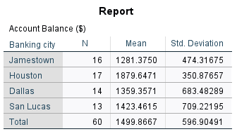
Guide: Read each city's N and Mean; the outcome is balance in dollars. Explanation: Houston has the largest observed mean ($1,879.65), followed by San Lucas ($1,423.46), Dallas ($1,359.36) and Jamestown ($1,281.38). This table alone does not test significance.
Guide: Compare bar heights on the dollar axis, not numeric city codes. Explanation: Houston has the highest sample mean. Use Q8's Welch/Games-Howell results to determine whether observed differences are statistically significant.
Question 02
ATM descriptive statistics by city
For each city, find the mean, median, mode, standard deviation, range, maximum, and minimum for number of ATM transactions per month.
Answer and analysis
Houston has the highest average ATM use (11.29 transactions per month). San Lucas is the most variable city (SD = 5.82; range = 18), and its mean (10.08) is above its median (8), reflecting the influence of higher-use customers. The multiple modes show that no city has a single uniquely most frequent transaction count.
| City | n | Mean | Median | All modes | SD | Range | Maximum | Minimum |
|---|---|---|---|---|---|---|---|---|
| Jamestown | 16 | 9.38 | 10.00 | 7, 10 | 3.44 | 13 | 17 | 4 |
| Houston | 17 | 11.29 | 12.00 | 6, 10, 12, 14 | 3.48 | 12 | 18 | 6 |
| Dallas | 14 | 10.00 | 9.50 | 7, 8, 12 | 4.17 | 15 | 17 | 2 |
| San Lucas | 13 | 10.08 | 8.00 | 6, 8, 14, 20 | 5.82 | 18 | 20 | 2 |
Guide: Read across each city row; the values are monthly ATM transaction counts. Explanation: All tied modes are shown, unlike SPSS's smallest-mode display. Mean/median describe typical use, while SD/range describe customer spread. Q2 requests descriptives, not a significance test.
Method and hypotheses
SPSS Frequencies is run separately for each city. Standard deviations are sample standard deviations. All tied modes are included in the summary below.
Checks and test selection
SPSS prints only the smallest mode when several values tie; its footnote is retained in the original table images.
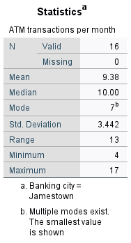
Guide: Read mean, median, mode, SD and range for Jamestown. Explanation: Its 16 customers average 9.38 ATM transactions; both 7 and 10 are modes. SPSS displays only the smallest tied mode, so the table below lists both.
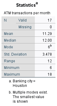
Guide: Read Houston's ATM summary and note the mode footnote. Explanation: The complete mode list is given in the combined table below. Mean and median describe location, while SD and range describe variation, not uncertainty in the mean.
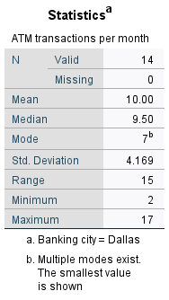
Guide: Read Dallas's ATM mean, median, smallest displayed mode and spread. Explanation: SPSS's tied-mode convention can omit other modes; use the combined table below for the full list. These values describe customers in Dallas, not a time trend.
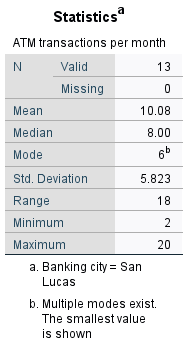
Guide: Read San Lucas's ATM mean, median, mode and spread. Explanation: Compare these with the other city summaries and the complete table below. A high range can reflect a small number of high-use customers rather than uniformly high use.
ATM distributions by city
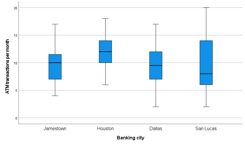
Guide: The line inside each box is the median; the box is the middle 50%, and markers identify potential outliers. Explanation: City ATM distributions differ in spread and high-use observations. This plot complements Q2; it is not a test of equal means.
The boxplots show medians, interquartile ranges, spread and potential outliers. They complement the mean, median, modes and ranges in the Q2 table; they do not replace those requested statistics. High-use observations help explain why some city means exceed their medians. The city labels are nominal codes, not numeric quantities.
Question 03
Account balance and receiving interest
Test if there is a significant difference between the Account Balance and Receive interest on the account.
Answer and analysis
Yes. Customers receiving interest have a higher mean balance ($1,693.50; SD = $282.51) than customers not receiving interest ($1,429.45; SD = $664.83). Welch’s two-sided t-test gives t(56.424) = -2.153, p = .036. Reject H0 at .05. The difference (no interest minus interest) is -$264.05 (95% CI: -$509.63 to -$18.46). Interest status is associated with balance, but this observational comparison does not show that receiving interest causes a higher balance.
Method and hypotheses
Independent-samples t-test comparing customers who receive interest with those who do not. H0: the two population mean balances are equal. H1: they differ.
Checks and test selection
Normality is not rejected: no-interest group (n = 44), Kolmogorov–Smirnov p = .200; interest group (n = 16), Shapiro–Wilk p = .077. Levene’s p < .001, so use the “Equal variances not assumed” (Welch) row.
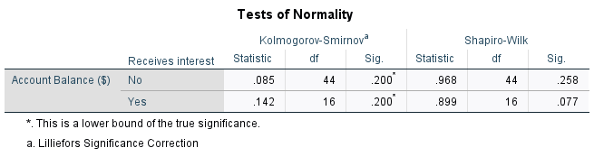
Guide: Apply the course sample-size rule separately to each interest group and compare Sig. with .05. Explanation: These normality checks are read alongside Q-Q plots. Failure to reject normality is not proof of normality; variance inequality determines the Welch row in Q3.
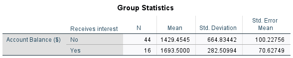
Guide: Read N, Mean, SD and SE for each interest group. Explanation: Interest-receiving accounts have the larger observed mean. Their mean difference is tested in the next table, rather than inferred from group summaries alone.

Guide: Read the Equal variances not assumed row, Sig. (2-tailed) and the difference CI. Explanation: Welch t(56.424) = -2.153, p = .036; no-interest minus interest is -$264.05 (95% CI -$509.63 to -$18.46). Reject equal means at .05.
Balance distributions by interest status
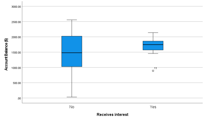
Guide: Compare medians, interquartile ranges, whiskers and outliers by interest status. Explanation: The different spreads support using a variance-robust comparison. The plot does not by itself prove a difference or an interest-payment effect.
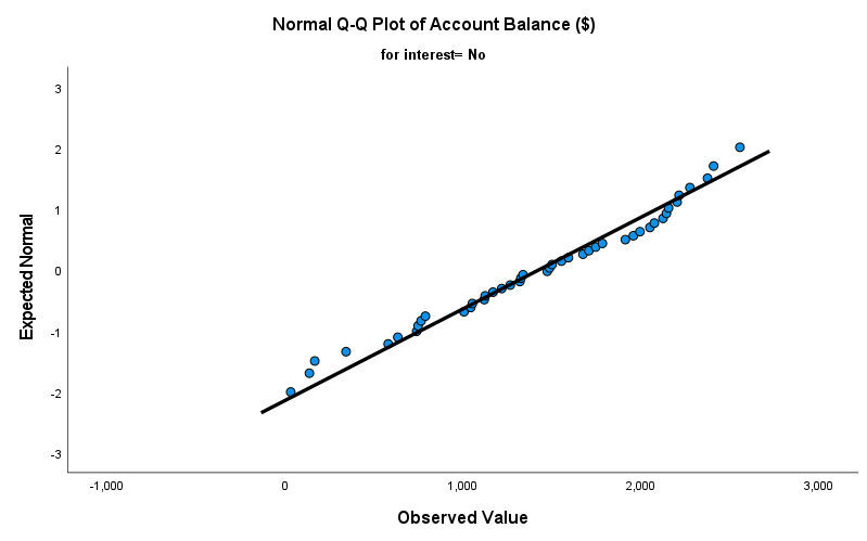
Guide: Compare no-interest balance points with the diagonal. Explanation: Departures show where the sample differs from a normal distribution. This visual check supplements the normality table; it cannot prove normality or establish independence.
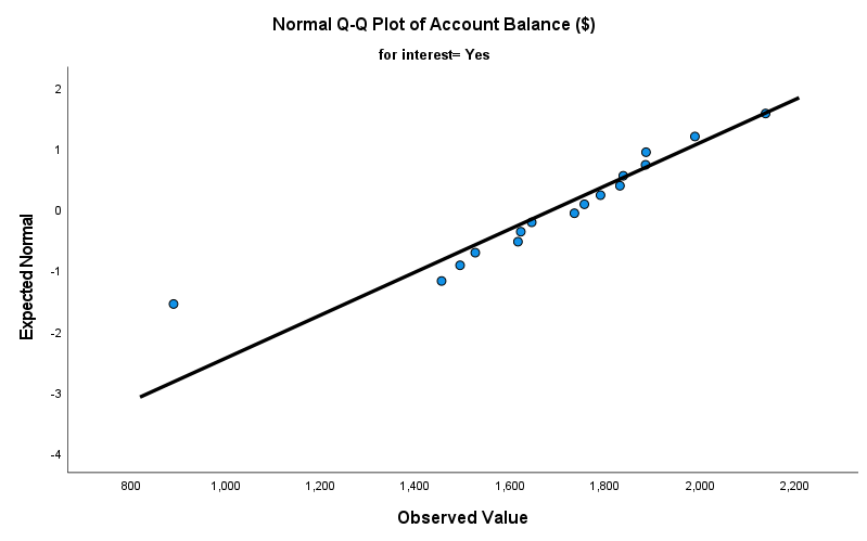
Guide: Compare interest-group balance points with the diagonal. Explanation: Interpret deviations together with group size and the normality test, not as an automatic pass/fail decision. Welch handles variance inequality, not every possible distribution problem.
The boxplot illustrates the different spreads that motivate the Welch row. The Q-Q plots supplement the normality test table. The visual contrast alone is not a significance test, and interest status is not a randomized treatment.
Question 04
Other bank services compared with seven
Test the hypothesis that the average of Number of other bank services used is equal to 7.
Answer and analysis
No. The sample mean is 4.42 services (SD = 1.98), significantly below 7: t(59) = -10.122, p < .001. Reject the mean-equals-7 hypothesis at .05. The estimated shortfall is 2.58 services (95% CI for mean minus 7: -3.09 to -2.07); the mean itself has a 95% CI of 3.91 to 4.93. The course-based Wilcoxon check also rejects its location/median benchmark (standardized statistic = -6.124, p < .001), supporting the direction of the finding. The bank could investigate barriers to using additional services rather than assume every customer needs seven.
Method and hypotheses
H0: the population mean number of other services is 7. H1: it is not 7. A two-sided one-sample t-test addresses this mean hypothesis, using a large-sample approximation (n = 60). A one-sample Wilcoxon test is also reported to follow the course’s non-normal-data branch.
Checks and test selection
Kolmogorov–Smirnov p = .002 rejects normality under the course rule for n > 30. These are discrete counts. The t-test therefore relies on the sampling-mean approximation, not on normally distributed individual counts. Wilcoxon evaluates a location/median benchmark under its symmetry assumption; it does not test the mean directly.
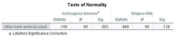
Guide: For all 60 service counts, read the course-selected Kolmogorov-Smirnov Sig. column. Explanation: Discrete service counts depart from normality, motivating the Wilcoxon sensitivity check. The required hypothesis about the mean remains distinct from a rank-location hypothesis.

Guide: Read the service-count N, Mean, SD and SE before testing against seven. Explanation: The sample mean is 4.42 services (SD 1.98), below the benchmark. Descriptive distance alone is not the inferential decision.
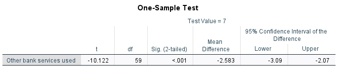
Guide: Test Value = 7; read t, df, two-sided p and the difference CI. Explanation: t(59) = -10.122, p < .001 rejects a population mean of seven. The negative difference indicates fewer services; the rank sensitivity result is explained separately.

Guide: Read the Wilcoxon hypothesis, Sig. and decision; its benchmark is seven. Explanation: It also rejects the benchmark (p < .001), but tests signed-rank location under its assumptions rather than the population mean directly.
Services distribution and signed ranks
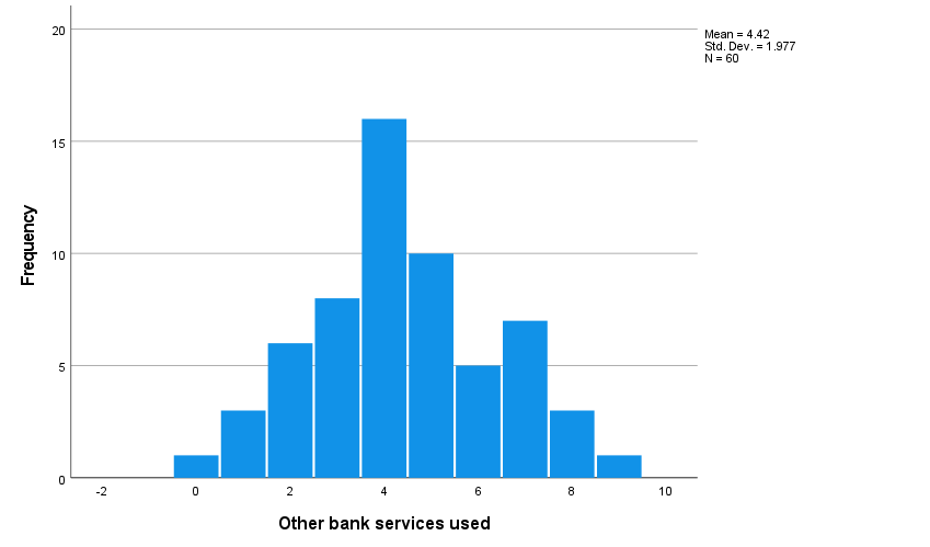
Guide: Read service-count values on the horizontal axis and customer frequencies vertically. Explanation: The histogram shows a discrete distribution concentrated below seven. It explains the normality concern but does not replace a significance test.
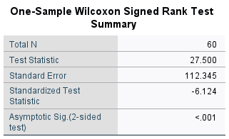
Guide: Read the standardized signed-rank statistic and two-sided significance. Explanation: Z = -6.124, p < .001 supports a location below seven. Symmetry is needed for the usual median/location interpretation; this is a sensitivity check, not a mean test.
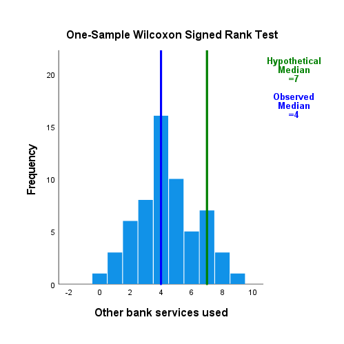
Guide: Compare the observed median line (4) with the hypothetical median line (7); bars show service frequencies, not means or signed ranks. Explanation: The lower observed median illustrates the test's direction. Significance comes from the Wilcoxon summary, not the distance between the lines.
The histogram displays the discrete service counts. The signed-rank visual compares values with the benchmark of seven; it accompanies the Wilcoxon summary already reported. Seven is a hypothesis benchmark, not a required number of services for each customer. The mean-based t-test and location-based rank test answer different statistical hypotheses.
Question 05
City and debit-card ownership
Test if there is a significance association between the "City where banking is done" and "whether or not the customer has a debit card".
Answer and analysis
No. There is no statistically significant evidence of an association between city and debit-card ownership: χ²(3, N = 60) = 0.224, p = .974. Fail to reject H0 at .05. Cramer’s V = .061 indicates a very small observed association. Debit-card ownership ranges from 38.5% in San Lucas to 47.1% in Houston; those sample differences do not establish different ownership rates in the populations. The bank should not base city-specific debit-card policies on these data alone.
Method and hypotheses
Pearson chi-square test of independence for a 4 × 2 contingency table. H0: city and debit-card ownership are independent. H1: they are associated.
Checks and test selection
Both variables are nominal. All expected cell counts exceed 5 (minimum = 5.63), so the chi-square approximation is appropriate, assuming independent customers.
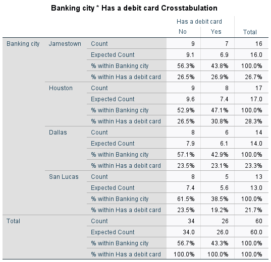
Guide: Compare observed with expected counts and distinguish row from column percentages. Explanation: City-debit counts total 60 customers. All expected cells exceed five, supporting the Pearson chi-square approximation; Q5 tests association, not differences in mean balances.
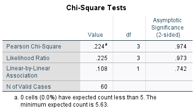
Guide: Read Pearson Chi-Square, df and Asymptotic Sig. (2-sided). Explanation: chi-square(3) = .224, p = .974, so there is no detected city-debit association. Failure to reject is not evidence that association is exactly zero.
City and debit-card ownership: chart
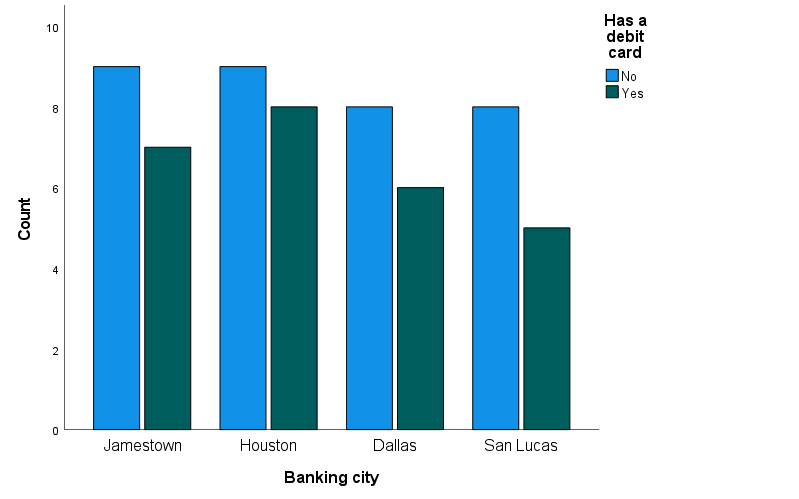
Guide: Bar height represents customer count; colors distinguish debit-card status within cities. Explanation: Similar observed proportions accompany the non-significant chi-square result. Unequal city totals mean raw bar heights should not be confused with ownership percentages.
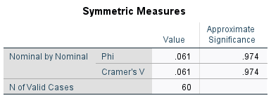
Guide: Read Cramer's V for the association's magnitude, alongside chi-square significance. Explanation: V = .061 is small in this sample. It measures categorical association, not a dollar difference or causal effect.
The chart shows counts, not ownership percentages. The city sample sizes differ (16, 17, 14 and 13), so compare ownership percentages as well as bar heights. Jamestown: 7/16 = 43.8%; Houston: 8/17 = 47.1%; Dallas: 6/14 = 42.9%; San Lucas: 5/13 = 38.5%. These figures are consistent with the non-significant chi-square result.
Question 06
Account balance and debit-card ownership
Test the hypothesis that “there is no significance between the Account Balance and whether or not a customer has a debit card.”
Answer and analysis
No. A significant balance difference is not detected: Mann–Whitney U = 415.000, Z = -0.403, SPSS two-sided p = .687. Fail to reject the distributional null hypothesis at .05. Mean balances are $1,435.82 without a debit card and $1,583.62 with one. The Welch mean comparison also fails to reject equality (p = .326); the mean difference (no card minus card) is -$147.79 (95% CI: -$446.23 to $150.65). These results do not prove the groups are identical; debit-card ownership alone is not a reliable basis for predicting balance here.
Method and hypotheses
The course-based analysis uses a two-sided Mann–Whitney U test because one group fails normality. H0: the balance distributions are the same in the two groups. A Welch t-test is included as a sensitivity check for the narrower question about equality of mean balances.
Checks and test selection
No-card group (n = 34): Kolmogorov–Smirnov p = .044, so normality is rejected. Card group (n = 26): Shapiro–Wilk p = .987. Mann–Whitney does not require normality, but its result cannot automatically be interpreted as a test of means or medians without additional distributional assumptions.
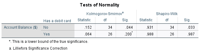
Guide: Read balance normality separately for customers with and without debit cards. Explanation: Distribution concerns motivate the Mann-Whitney analysis. Its rank hypothesis is distinguished from the Welch sensitivity test of population means.
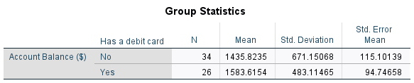
Guide: Compare debit groups' N, Mean, SD and SE. Explanation: These summarize dollar balances, while the following Mann-Whitney table uses ranks. A visible difference in group means does not alone establish statistical significance.
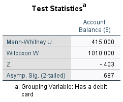
Guide: Read Mann-Whitney U, Z and two-sided significance. Explanation: U = 415, Z = -.403, p = .687: no distribution/rank difference is detected. This is not automatically a test that mean balances are equal.

Guide: Read the unequal-variances row to test the mean-based interpretation of Q6. Explanation: Welch p = .326 also fails to detect a mean difference. Neither a non-significant t-test nor rank test proves equivalence.
Debit-card balance ranks and distribution
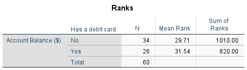
Guide: Mean Rank and Sum of Ranks describe ordered balances, not dollars. Explanation: Mean ranks are 29.71 without a card and 31.54 with a card; the U test finds this separation non-significant (p = .687).
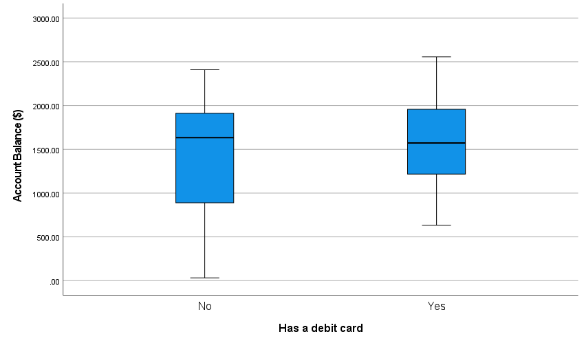
Guide: Compare debit-group medians, boxes, whiskers and potential outliers. Explanation: The distributions overlap substantially and spreads differ. The plot illustrates the data; use the U and Welch tests for their respective statistical hypotheses.
The mean ranks are 29.71 without a debit card and 31.54 with a card. The ranks and boxplot accompany the Mann–Whitney test, as in Lecture 14. The large overlap and unequal spreads make it inappropriate to claim a clear separation of balance distributions or interpret the rank test as an automatic test of mean balances.
Question 07
Account balance compared with $2,000
Test the hypothesis that the average Account Balance is equal 2000 $.
Answer and analysis
No. The estimated mean balance is $1,499.87 (SD = $596.90), significantly below $2,000: t(59) = -6.490, p < .001. Reject H0 at .05. The estimated mean difference is -$500.13 (95% CI: -$654.33 to -$345.94), and the mean balance has a 95% CI of $1,345.67 to $1,654.06. For planning based on customers like this sample, using $2,000 as the expected average would overstate observed balances.
Method and hypotheses
Two-sided one-sample t-test. H0: the population mean account balance is $2,000. H1: it differs from $2,000.
Checks and test selection
For n = 60, Kolmogorov–Smirnov p = .176 does not reject normality under the course rule. Shapiro–Wilk p = .063 also does not reject normality. Independence and a representative sample are needed for population inference.
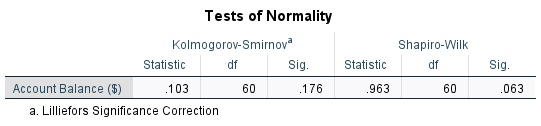
Guide: For the 60 balance observations, read the course-selected Kolmogorov-Smirnov significance alongside Q-Q output. Explanation: The distribution check informs interpretation of the one-sample t-test. No normality test can verify the sampling independence assumption.
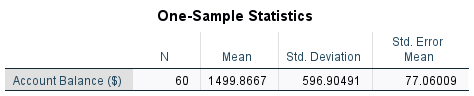
Guide: Read overall N, Mean, SD and SE in dollars. Explanation: The 60-customer mean is $1,499.87 (SD $596.90). The next table tests the difference from $2,000; SD is customer spread, while SE is mean precision.
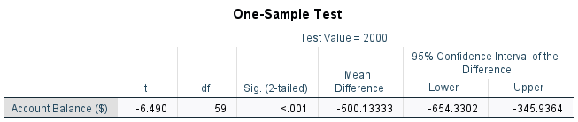
Guide: Test Value = $2,000; read t, df, p and Mean Difference. Explanation: t(59) = -6.490, p < .001 rejects the benchmark. The sample mean is about $500.13 lower; the test does not predict every customer's balance.
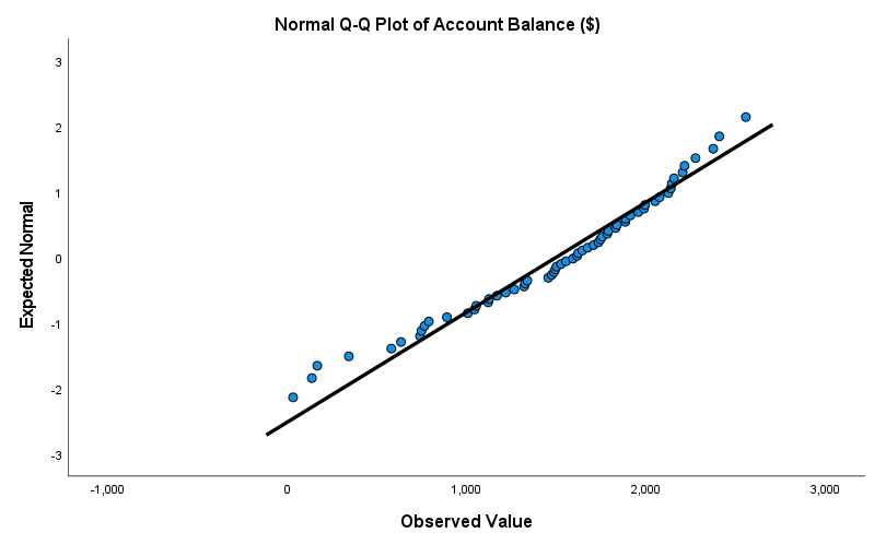
Guide: Compare the balance quantiles with the reference line, especially the tails. Explanation: The Q-Q plot supplements the normality test for Q7. Modest visual departures do not justify ignoring sampling design or treating the t-test as a causal analysis.
Question 08
One-way ANOVA of account balance across cities
Test if there is a significant difference between the average Account Balance for the different cities.
Answer and analysis
Yes. Welch ANOVA shows that at least one city mean differs: F(3, 28.026) = 6.521, p = .002. Reject H0 at .05. Games–Howell identifies Houston as significantly higher than Jamestown by $598.27 (p = .002; 95% CI: $199.39 to $997.16). No other city pair is significant at .05 after these comparisons. Houston has the highest observed mean, but the result does not establish that banking in Houston causes higher balances; customer composition and other factors could explain the difference.
Method and hypotheses
One-factor comparison of four independent city groups. H0: all four population mean balances are equal. H1: at least one differs. Use Welch one-way ANOVA and Games–Howell post-hoc comparisons because variances are unequal.
Checks and test selection
Each city has fewer than 30 customers. Shapiro–Wilk p-values are .543 (Jamestown), .839 (Houston), .257 (Dallas) and .936 (San Lucas); normality is not rejected. Levene’s p = .040 rejects equal variances. The ordinary pooled ANOVA row is therefore not the primary test.
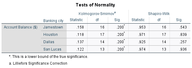
Guide: Each city has fewer than 30 cases, so read its Shapiro-Wilk Sig. value. Explanation: These small-group checks do not reject normality, but have limited power. Levene's result, rather than normality alone, motivates Welch ANOVA.
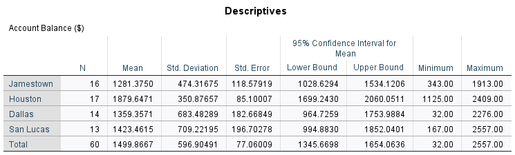
Guide: Read city N, mean, SD, SE and mean CI. Explanation: Houston has the highest sample mean; the four group sizes and spreads are not identical. These descriptive intervals are separate from adjusted pairwise comparison intervals.
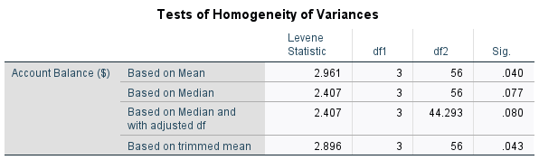
Guide: Read the mean-based Levene row and compare Sig. with .05. Explanation: p = .040 rejects equal city variances. Use Welch for the omnibus mean comparison and Games-Howell for pairwise comparisons rather than pooled-variance Tukey.
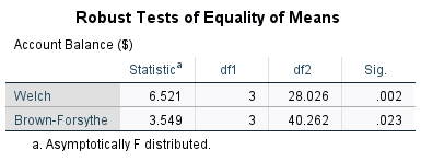
Guide: Read the Welch row, Statistic, both degrees of freedom and Sig. Explanation: F(3, 28.026) = 6.521, p = .002 rejects equal city mean balances. An omnibus result says at least one mean differs, not that every pair differs.
City mean comparisons: Games–Howell
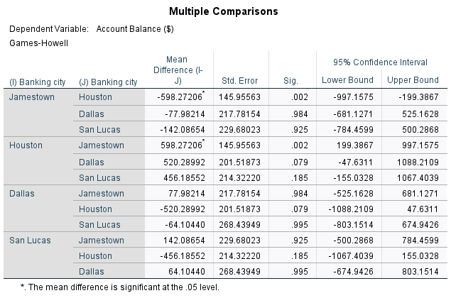
Guide: Use the Games-Howell Sig. column and each pair's 95% CI. Explanation: Only Houston-Jamestown is significant (p = .002), with Houston about $598.27 higher (CI $199.39 to $997.16). Other city pairs are not significant at .05.
The significant pair is Houston–Jamestown. Houston–Dallas has p = .079 and Houston–San Lucas has p = .185, so neither is significant at .05. An omnibus difference does not imply that every city differs from every other city. The repeated reverse-direction rows are the same comparisons with opposite signs; they are not additional independent findings.
Ordinary ANOVA and city mean confidence intervals
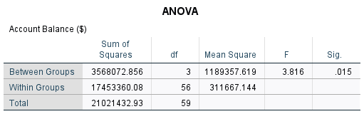
Guide: Read the ordinary ANOVA F, df and Sig., then check its variance assumption. Explanation: F(3, 56) = 3.816, p = .015 is shown for lecture coverage. Because Levene p = .040, Welch remains the primary result.
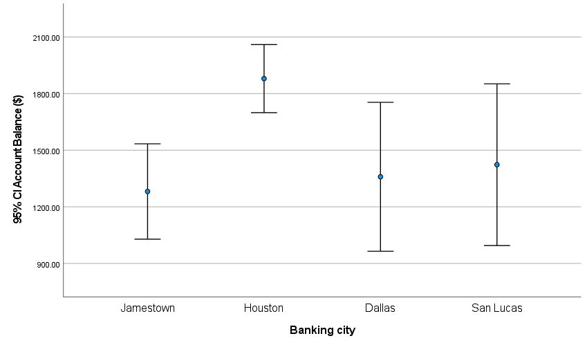
Guide: Points/bars show city means; error bars are individual 95% confidence intervals, not +/-1 SD or SE. Explanation: Houston has the largest estimated mean. CI overlap is not an adjusted pairwise test; use Games-Howell for pair decisions.
The lecture-style ordinary one-way ANOVA gives F(3, 56) = 3.816, p = .015. It is shown for completeness, but its equal-variance assumption is rejected (Levene p = .040), so Welch F(3, 28.026) = 6.521, p = .002 remains the primary result. The plotted intervals describe each city mean separately. Their overlap is not the Games–Howell pairwise test; use the adjusted comparison table for pairwise significance. Tukey is not used because it pools the unequal variances.
Kruskal–Wallis sensitivity and pairwise comparisons
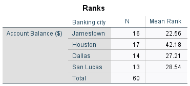
Guide: Read each city's Mean Rank and N rather than interpreting ranks as dollars. Explanation: Houston's mean rank is highest (42.18), while Jamestown's is lowest (22.56). The next table tests the omnibus rank difference.
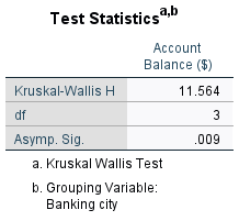
Guide: Read Kruskal-Wallis H, df and significance. Explanation: H(3) = 11.564, p = .009 detects a city distribution/rank difference. This sensitivity analysis is not interchangeable with Welch's hypothesis about means.
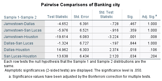
Guide: Read Adj. Sig., not the unadjusted Sig., for the six city pairs. Explanation: After Bonferroni adjustment, only Jamestown-Houston is significant (p = .008). Adjustment controls the familywise error across these pairwise comparisons.
The rank-based sensitivity analysis gives H(3) = 11.564, p = .009. It also detects a city difference, but tests balance distributions/ranks rather than equal means. The Bonferroni-adjusted pairwise result is significant only for Jamestown–Houston (p = .008); Houston has the higher mean rank. Use the Adj. Sig. column, not the unadjusted Sig. column.
Rank pairwise comparison diagram
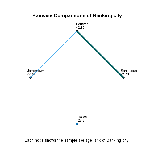
Guide: Node labels show cities' mean ranks; consult the adjusted table to interpret pairwise significance. Explanation: Houston-Jamestown is the only significant adjusted pair. Lines and node positions do not represent geography, dollar differences or causation.
Each city node shows its mean rank: Houston 42.18, San Lucas 28.54, Dallas 27.21 and Jamestown 22.56. These are ranks, not dollar balances. The adjusted pairwise table identifies only Houston–Jamestown as significant (p = .008); the other city comparisons are not significant at .05. The diagram complements the table and does not imply causation or geographical distance.
Exploratory two-way ANOVA of city and debit-card status
This extension jointly examines the factors used in Q6 and Q8. Account balance is the outcome; city has four levels and debit-card ownership has two. The full factorial Type III model tests city, debit status and their interaction. It is supplementary to the ten specified questions, not a replacement for their unadjusted tests.
All eight cells contain 5–9 customers. Shapiro–Wilk does not reject cell normality (p = .186 to .961), but these small cell samples have limited power. Mean-based Levene gives F(7, 52) = 2.799, p = .015, so conventional pooled-variance F tests and confidence intervals require caution. The variance-appropriate Welch/Games–Howell analysis remains the main conclusion about cities.
The conventional two-way ANOVA detects a city main effect, F(3, 52) = 3.588, p = .020, partial eta squared = .172. It does not detect a debit-card main effect, F(1, 52) = 1.370, p = .247, or a city × debit-card interaction, F(3, 52) = 1.738, p = .171. The profile lines are not parallel, but that visual pattern is not statistically significant evidence of interaction. Estimated marginal city means give equal weight to the two debit groups; they therefore differ slightly from the raw city means in Q1/Q8. These observational and heteroscedastic results do not establish causal effects.
Factorial descriptives and assumption checks
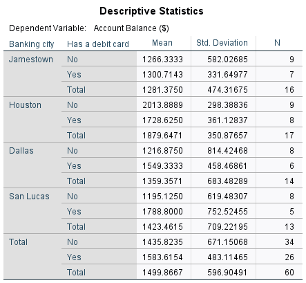
Guide: Read N, mean and SD for each city-by-debit cell. Explanation: All eight cells are populated, with 5-9 customers each. Small cells make distribution checks weak and estimated interactions less stable than a large factorial sample.
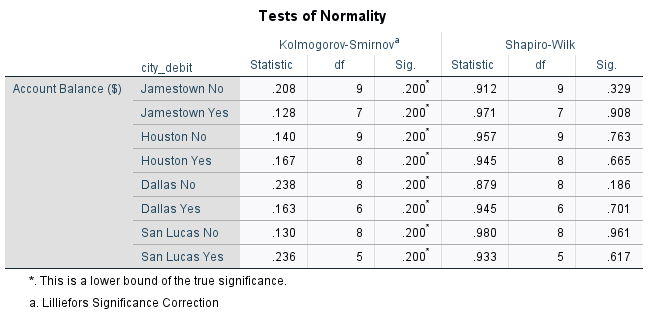
Guide: Read Shapiro-Wilk for each of the eight cells. Explanation: All p-values are .186-.961, so normality is not rejected. With only 5-9 cases per cell, this is limited evidence; the unequal-variance finding still warrants caution.
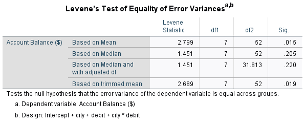
Guide: Read Levene F, df and Sig. for the eight-cell factorial model. Explanation: F(7, 52) = 2.799, p = .015 rejects equal cell variances. Conventional Type III F tests and pooled-model CIs are therefore exploratory, not the main city conclusion.
Factorial ANOVA and estimated marginal means
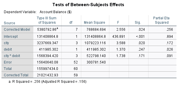
Guide: Read city, debit and city x debit rows, their F, Sig. and partial eta-squared. Explanation: City p = .020; debit p = .247; interaction p = .171. Only the city effect is detected, and heteroscedasticity limits the conventional model's inference.
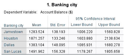
Guide: Estimated marginal city means average the two debit groups with equal weights. Explanation: They differ slightly from raw Q1 means because group sizes differ. Their model-based CIs assume the conventional factorial variance model and require caution.
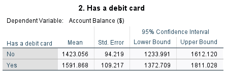
Guide: Estimated debit-group means average across the four cities with equal weights. Explanation: These are adjusted model summaries, not raw group averages. The debit main-effect test is non-significant (p = .247); do not infer significance from plotted or tabulated means alone.
City × debit-card interaction profile
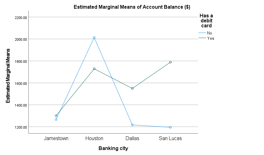
Guide: Follow debit-group profile lines across nominal city categories, not time. Explanation: Nonparallel lines suggest a possible interaction visually, but the interaction test is not significant (p = .171). This plot cannot establish city or debit causal effects.
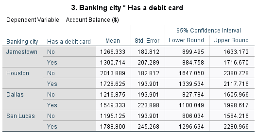
Guide: Read each city-debit estimated mean, SE and 95% CI. Explanation: These describe the eight model cells, not eight independent significance decisions. Small cell sizes and unequal variances make the pooled-model intervals exploratory.
Question 09
Excel correlation: balance and ATM transactions
Using Excel, find the correlation coefficient between the Account Balance and Number of ATM transactions per month? Interpret your result.
Answer and analysis
There is a strong positive linear relationship: r = 0.70499 (approximately .705), n = 60, p < .001. Customers with more ATM transactions tend to have higher account balances in this sample. The squared correlation is about .497, so the single-predictor linear relationship accounts for about 49.7% of the observed balance variation. The plotted trendline uses ATM alone; it is not the two-predictor equation in Question 10. Association does not establish that increasing ATM transactions will increase a customer’s balance.
Method and hypotheses
Pearson correlation calculated in Microsoft Excel: =CORREL(Data!A2:A61,Data!B2:B61). Both variables are quantitative, and the scatterplot is used to assess the direction and approximate linear form.
Checks and test selection
The calculation includes all 60 customer pairs. Correlation describes a linear relationship; independent observations and the usual inferential assumptions are needed for its p-value. The course classifies a correlation above .70 as strong.
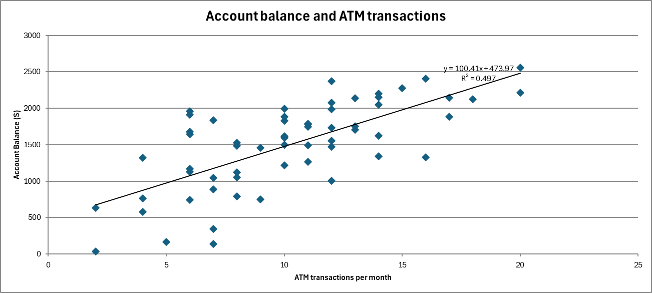
Guide: Each point is one customer's ATM use and dollar balance; the fitted line summarizes their linear relationship. Explanation: The positive trend accompanies r = .70499 and simple-model R-squared about .497. This line is not the two-predictor model used for Q10.
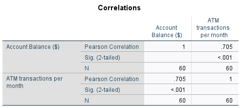
Guide: Read Pearson Correlation, Sig. (2-tailed) and N for balance versus ATM use. Explanation: r = .70499, p < .001, N = 60 indicates a strong positive linear association under the lecture's convention. SPSS checks the Excel result, but Q9 is calculated in Excel.
Question 10
Excel multiple regression and prediction
Using Excel, estimate: Account Balance = a + b (Number of ATM transactions) + c (Number of other bank services used). (i) Write the linear equation of the model. (ii) Predict Account Balance when ATM transactions per month = 15 and other bank services used = 4.
Answer and analysis
(i) Predicted Account Balance ($) = 247.0307 + 93.1334 × ATM transactions + 68.2241 × other services. (ii) At 15 ATM transactions and 4 services, the predicted balance is $1,916.93, using the unrounded Excel coefficients. Holding the other predictor constant, one additional ATM transaction is associated with $93.13 higher predicted balance, and one additional service with $68.22. The model is significant, F(2, 57) = 34.200, p < .001; R² = .545 and adjusted R² = .530. ATM has p < .001 and services p = .017. The prediction is an estimated conditional mean, not a guaranteed individual balance; residual standard error is about $409.43. These coefficients are associations, not causal effects.
Balance = 247.0307 + 93.1334 × ATM + 68.2241 × services
Method and hypotheses
Ordinary least-squares multiple regression calculated in Microsoft Excel using LINEST with an intercept: =LINEST(Data!A2:A61,Data!B2:C61,TRUE,TRUE). LINEST returns predictor coefficients in reverse column order, so the services and ATM coefficients are assigned to the correct variables. Excel t- and F-distribution formulas calculate inference.
Checks and test selection
The predictors are ATM transactions and other services, not the numeric city or yes/no codes. SPSS model output and residual plots accompany the Excel results. The requested input values (15 ATM transactions, 4 services) are within the observed ranges.
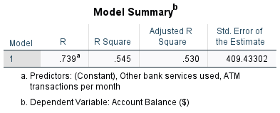
Guide: Read R-squared, adjusted R-squared and Std. Error of the Estimate. Explanation: The two predictors explain about 54.5% of sample balance variation (adjusted 53.0%); residual SE is about $409.43. Explained variation is not prediction certainty.
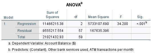
Guide: Read regression F, model/residual df and Sig. Explanation: F(2, 57) = 34.200, p < .001 rejects the hypothesis that both predictor slopes are zero. This regression ANOVA is different from the city-group ANOVA in Q8.
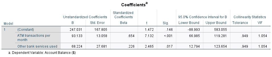
Guide: Use Unstandardized B for the equation; t, Sig. and CI describe each slope holding the other predictor fixed. Explanation: Balance = 247.0307 + 93.1334 x ATM + 68.2241 x services. At 15 and 4, Excel predicts $1,916.93 using unrounded coefficients.
Regression diagnostics
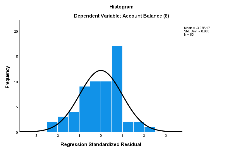
Guide: Read the distribution of standardized residuals, not raw balances. Explanation: There is no pronounced non-normal pattern, but a histogram is only a visual diagnostic. Approximate residual normality supports conventional regression inference, not causal claims.
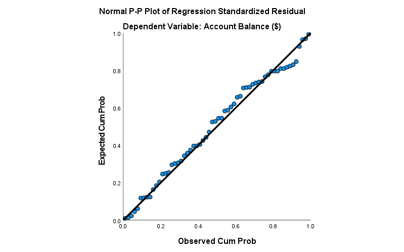
Guide: Points close to the diagonal indicate residual probabilities near a normal reference. Explanation: No pronounced systematic departure appears. The P-P plot supplements the histogram; it does not establish independence or constant variance.
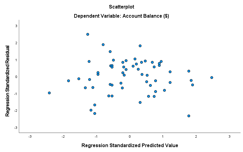
Guide: Look for curvature, a widening funnel or isolated extreme points around zero residual. Explanation: No obvious strong curve or funnel appears, though this cannot prove linearity/homoscedasticity. Sampling independence still requires study-design information.
The residual histogram and P-P plot show no pronounced departure from approximate normality. The residual-versus-fitted plot shows no obvious curved pattern or strong funnel, although visual checks cannot prove linearity or constant variance. Both VIFs are 1.054, so there is little evidence of multicollinearity. Standardized residuals range from -2.337 to 2.481 and maximum Cook’s distance is .196: no case exceeds the conventional Cook’s-distance threshold of 1, but influential cases still deserve review. Independence cannot be established from these plots; sampling and collection details remain important.